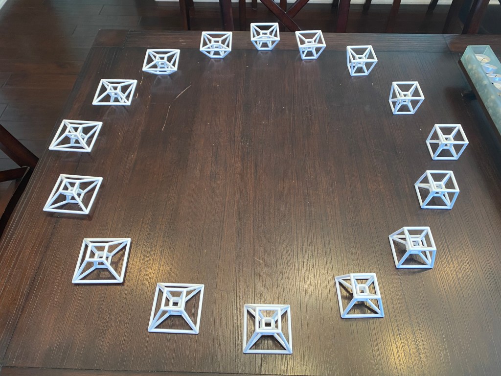
3D-printed models of a hypercube’s “shadow” during its double rotation in 4-dimensional space, designed in Mathematica

Background

This project is part of my Zoetrope of a Rotating Hypercube’s Shadow piece, which is a work in progress.

Introduction

The hypercube, also known as a tesseract, is the 4-dimensional analog of a “cube”. It’s not something that can be visualized whole by those of us who are creatures of a 3-dimensional universe. However, it is possible to glean a basic understanding of the hypercube’s structure (and 4-dimensional space, more generally), by observing 3-dimensional “shadows” of the object as it tumbles around in 4-space. The particular type of “tumbling” we’re interested in, illustrated in the graphic below, is known as double rotation — a transformation which (literally) doesn’t have a 3-dimensional equivalent.

**Figure 1.** The projection of a hypercube rotating in 4-space.
Credit: Jason Hise, CC0, via Wikimedia Commons

Note: You might be able to clearly distinguish between the two very different rotations in this double rotation. One of them appears quite “normal”, while the other is manifested in what looks like the object continually passing through itself. This is just an artifact of our inability to visually conceive movement in the $w$ -direction.

The goal of this project is to produce a sequence of 3-dimensional objects that can be combined through a stop-motion sort of process to animate the smooth kinetic flow of the hypercube performing a double rotation. Since the movement is clearly periodic (it repeats itself after some time), only a handful of these objects are necessary in order to create an apparition of fluid (and endless) motion.

In the next sections, I’ll discuss the mathematical concepts used to describe the hypercube, its double rotation, and its projection to 3-dimensional space; the modeling process (using Mathematica); and the “slicing” and 3D printing process.

Main concepts

First, since a hypercube is native to a higher-dimensional space, we will discuss what is meant by the mathematical notion of dimension, and how it is used to encode and utilize information about the hypercube and its shadows. Next, we will formalize what is meant by rotation. Specifically, we will discuss how the sine and cosine functions are used to express double rotation as a matrix transformation. Lastly, we’ll cover the mathematics of “shadows” (more formally known as projections), and learn how to find a higher-dimensional object’s 3-dimensional shadow by solving simple equations.

Dimension

The best way to understand the ambient (spatial) dimension of a space is to count its fundamental directions of motion. In 3-dimensional space, we have three: right-left, forward-backward, and up-down. A creature living in Edwin A. Abbott’s Flatland would only recognize two fundamental directions. And, extending the concept, it must be the case that 4-dimensional space has an additional degree of freedom which is entirely independent of the three we know. These directions are often called ana (in the positive direction) and kata (in the negative one), terms which were apparently first used in Charles Howard Hinton’s A New Era of Thought.

We can describe 4-dimensional space using the Cartesian coordinate system with four mutually-perpendicular coordinate axes, which we’ll call $x$ , $y$ , $z$ , and $w$ — the $w$ -axis usually referring to the ana-kata direction. that means that a point with coordinates $(1, 2, -2, 1)$ is located 1 unit to the right, 2 units in front of, 2 units underneath, and 1 unit ana of the origin (in your frame of reference).

In order to gain an intuition for the structure of 4-dimensional space and the objects it contains, we shall consider the generalization of very simple geometric object: the “cube”. Why a cube? Well, the cube is, in some sense, the essence of 3-dimensionality. A solid box with equal side lengths, it inhabits space uniformly in each of three independent (even better: perpendicular) spatial directions. In fact, there is a notion for “cube” in each ambient spatial dimension. Keep in mind that each of these objects is solid, containing not only its boundary, but its “insides” (e.g. the square is filled in).

0-cube: point, 0-dimensional (nothing to measure!)
1-cube: line segment, 1-dimensional, measured in length
2-cube: square, 2-dimensional, measured in area
3-cube: cube (yes, the one you’re thinking of), 3-dimensional, measured in volume
4-cube: hypercube, 4-dimensional, measured in “hypervolume” (volume times length)

It’s a really lovely mental excursion to think about how the sequence of n-cubes builds on itself. This process is illustrated for the comprehensible directions in the following graphic, but the construction certainly generalizes into higher dimensions.

**Figure 2.** Constructing n-cubes. Image by the author.

Without being able to visualize it, we should be able to confidently say that the 4-cube is obtained by extending the solid 3-cube into the ana and kata directions. This fact can be used to explicitly write down the vertices of the hypercube which follows the sequence illustrated in Figure 3:

(0, 0, 0, 0), (1, 0, 0, 0), (0, 1, 0, 0), (1, 1, 0, 0), (0, 0, 1, 0), (1, 0, 1, 0), (0, 1, 1, 0), (1, 1, 1, 0)
(0, 0, 0, 1), (1, 0, 0, 1), (0, 1, 0, 1), (1, 1, 0, 1), (0, 0, 1, 1), (1, 0, 1, 1), (0, 1, 1, 1), (1, 1, 1, 1)

This list contains 16 vertices: two sub-lists of eight vertices, each sub-list corresponding to one copy of the 3-cube which was extended into the ana-kata direction. Note that the first three coordinates of each point in the first row are the same as the first three coordinates of the corresponding point in the second row — this pattern is an artifact of the 3-cube’s extension into 4-space, and it manifests itself in the hypercube’s geometry as edges.

Rotation

Regardless of the ambient space, rotation is a transformation which occurs “in the plane”. To understand why, consider that rotation is essentially motion along a circular path, and any circle lies in some plane. This means that rotation doesn’t make sense in Lineland (because of insufficient dimensionality). But in in Flatland, rotation is a transformation around a point. For objects in (3-dimensional) space, rotation happens around a line. So this means that we should expect rotation in 4-dimensional space to occur around a plane (a motion that you should not be able to visualize with your 3-dimensional perspective). And, indeed, this turns out to be the precisely the case.

To see how this all works out mathematically, let’s start with a lower-dimensional case. Some of you will recognize the function

$\mathbf{R}_2(\theta)=\begin{bmatrix}\cos(\theta) & -\sin(\theta)\\\sin(\theta) & \cos(\theta)\end{bmatrix}$

as a linear (matrix) transformation which rotates points in the $xy$ -plane through an angle of $\theta$ (radians) in the counter-clockwise direction around the origin. Specifically, this matrix transformation acts through left-multiplication, like so:

$\begin{bmatrix}\cos(\theta) & -\sin(\theta)\\\sin(\theta) & \cos(\theta)\end{bmatrix}\cdot\begin{bmatrix}x_0\\y_0\end{bmatrix}=\begin{bmatrix}x_1\\y_1\end{bmatrix}$

Note that $\begin{bmatrix}x_1\\y_1\end{bmatrix}$ is the rotation of $\begin{bmatrix}x_0\\y_0\end{bmatrix}$ . The same idea extends to matrix action in higher dimensions.

And since rotation is always a transformation which occurs “in the plane”, we can extend the above definition of $\mathbf{R}_2(\theta)$ to higher-dimensional spaces. In particular,

$\mathbf{R}_3(\theta)=\begin{bmatrix}\cos(\theta) & -\sin(\theta) & 0\\\sin(\theta) & \cos(\theta) & 0\\ 0 & 0 & 1\end{bmatrix}\phantom{XX}\text{and}\phantom{XX} \mathbf{R}_4(\theta)=\begin{bmatrix}\cos(\theta) & -\sin(\theta) & 0 & 0\\\sin(\theta) & \cos(\theta) & 0 & 0\\ 0 & 0 & 1 & 0\\ 0 & 0 & 0 & 1\end{bmatrix}$

are also matrices which encode rotation in in the $xy$ -plane. However, $\mathbf{R}_3(\theta)$ is defined for objects in 3-space (and fixes the $z$ -axis), while $\mathbf{R}_4(\theta)$ is defined in 4-space (and fixes both the $z$ – and $w$ -axes).

Using the same idea to encode rotation in the $zw$ -plane as

$\mathbf{R}'_4(\theta)=\begin{bmatrix}1 & 0 & 0 & 0\\0 & 1 & 0 & 0\\0 & 0 & \cos(\theta) & -\sin(\theta)\\0 & 0 & \sin(\theta) & \cos(\theta)\end{bmatrix}$

it’s now possible to express a double rotation in 4-space, occurring (at the same rate) in the $xy$ – and $zw$ -planes, as the transformation defined by the following matrix function:

$\mathbf{DubRot}(\theta) = \mathbf{R}_4(\theta)\cdot\mathbf{R}'_4(\theta)=\begin{bmatrix}\cos(\theta) & -\sin(\theta) & 0 & 0\\\sin(\theta) & \cos(\theta) & 0 & 0\\0 & 0 & \cos(\theta) & -\sin(\theta)\\0 & 0 & \sin(\theta) & \cos(\theta)\end{bmatrix}$

The fact that this matrix is block-diagonal reinforces the disjoint quality of the two rotations which compose the double rotation.

Projection

Projection is the mathematical concept which explains the phenomenon of a shadow. Projection is essentially a “flattening” operation, reducing the dimension of the object. The two types of projections I’d like to mention (there are many more) are akin to the two types of shadows: those made by an overhead lamp versus those made by the mid-day sun. The difference between the two is evident in the fact that a shadow made by the sun at noon doesn’t warp dimensions or angles like a shadow cast by an overhead lamp. This is because light from the sun is essentially an “infinite” distance away from the object it shadows (yes, it makes me cringe to even suggest that a very measurable length is infinite, by the way, but this observation is a common one), so as to illuminate the object with parallel light rays. This is not the case with light coming from a lamp, no matter how tall it is. An object’s shadow cast by lamp light will have a characteristic distortion, which provides a sense of depth which is not evident in sunlight shadows.

Both types of projections discussed above are illustrated in this interactive GeoGebra applet, a screenshot of which is given in Figure 3 below. Note that the illustrated setting is a direct lower-dimensional analog of the one we’re interested in modeling: a 3-dimensional shadow of a 4-dimensional object.

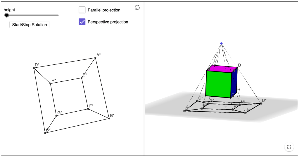
**Figure 3.** Screenshot of an interactive GeoGebra applet illustrating both parallel and perspective projections. Applet and image by the author.

It turns out that a parallel projection along perpendicular axes is much simpler to model since the “extra dimension” is essentially squashed. We can easily accomplish this with the following matrix transformation:

$\mathbf{Proj}_{\infty}=\begin{bmatrix}1&0&0&0\\0&1&0&0\\0&0&1&0\end{bmatrix}$

As suggested by Figure 3, perspective projection is defined relative to some point (analogous to a shadow’s light source), located outside of the lower-dimensional space onto which we wish to project. To find a object’s “shadow” cast from this perspective point, we consider the collection of lines passing through the perspective point and each of the object’s vertices. The points at which these lines intersect the lower-dimensional space define the vertices of the object’s projection.

Recall that if $P$ and $Q$ are two distinct points in the same ambient space, then there is a unique line passing through both $P$ and $Q$ — hopefully you remember this fact from your first geometry course. And, regardless of dimension, we can represent this line using the parametric function $L(t)=tQ+(1-t)P$ , where the parameter $t$ ranges through all real numbers. In particular, note that $L(0)=P$ and $L(1)=Q$ . Points along the line which are between $P$ and $Q$ correspond to $0<t<1$ . Points on the line “before” $P$ correspond to $t<0$ , and points “after” $Q$ correspond to $t>1$ .

Now, if $P$ and $Q$ are points in $\mathbb{R}^4$ , then the line between them will naturally decompose as $L(t)=(x(t), y(t), z(t), w(t))$ . Therefore, the intersection of the line with $\mathbb{R}^3$ (which is defined by $w=0$ ) can be found by:

Solving the equation $w(t)=0$ , which determines when the intersection occurs.
Then evaluating the function $L(t)$ at this solution, determining where the intersection occurs.

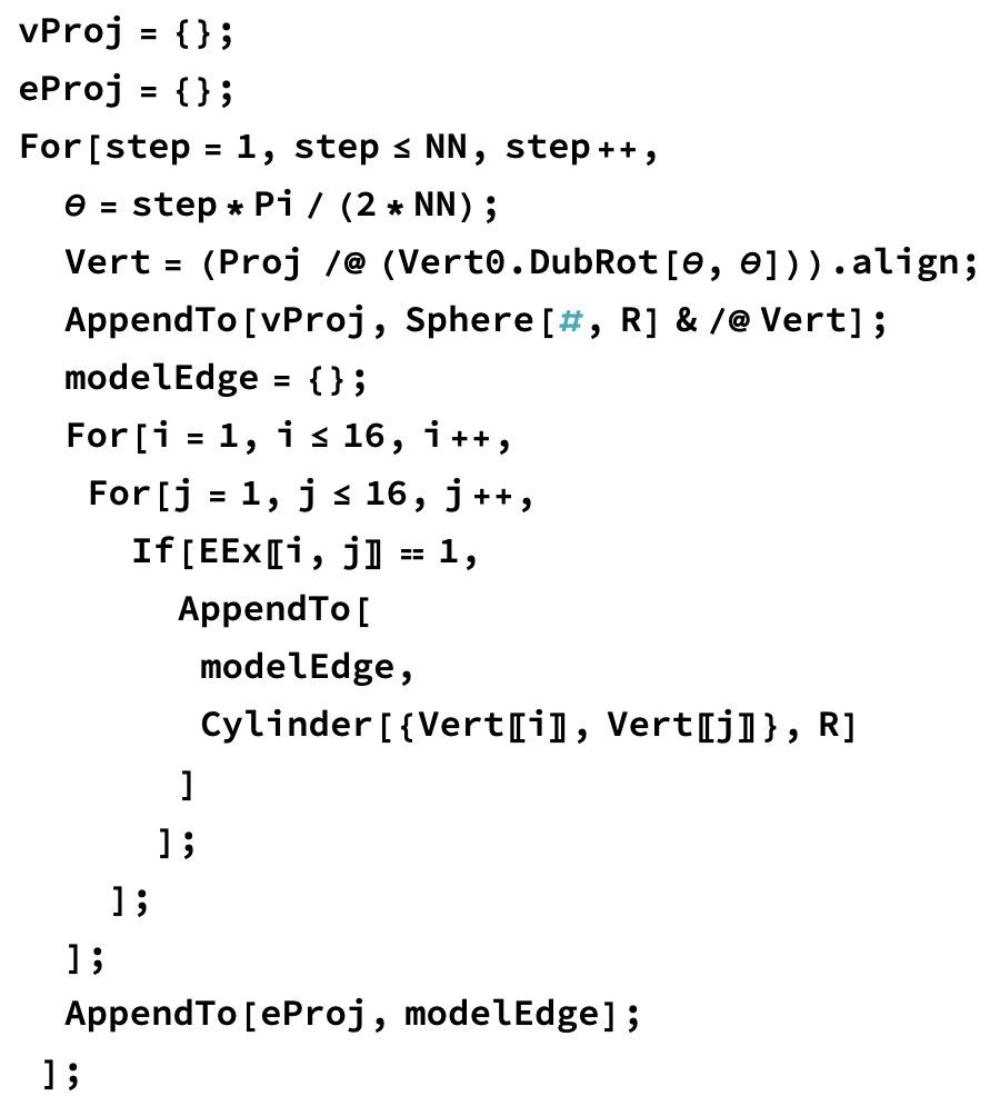
For the sake of simplicity, we take our perspective point (which we’ll call $P$ ) to be located along the $w$ -axis (just as the perspective point in Figure 3 is located along the $z$ -axis). To find the projection of the hypercube onto $\mathbb{R}^3$ from the perspective of $P$ , we simply follow the short algorithm described above for each vertex $Q\in\mathbb{R}^4$ of the hypercube.

Modeling

The 3D-modeling for this project was performed using Mathematica. The online notebook, containing all source code and rich in-line documentation, can be accessed with a Wolfram ID (which is free with their Cloud Basic account).

**Figure 4.** A portion of the Mathematica script which defines the structure of each hypercube shadow model. Image by the author.

Production

The final phase of the project involves converting each model’s STL encoding into a tangible (plastic) object that you can place on your bookshelf or hang from your rear view mirror. There are two steps involved in production: slicing (i.e. preparation for printing) and 3D printing.

Slicing

Slicing is a process which takes an STL file and creates a very specific step-by-step procedure (called G-code) that the 3D printer should follow in order to produce the encoded model. In other words, slicing converts the model’s format into a language that the printer understands.

There are many open-source slicers out there; I use PrusaSlicer because (1) its presets are well-tuned for my Prusa hardware (details below), and (2) it came highly recommended by the 3D printing community.

**Figure 5.** The PrusaSlicer interface in action. Image by the author.

The slicing process allows for a myriad of print setting customizations (that would lead me down a rabbit hole if I paused to elaborate on), but I only ended up making significant adjustments to the support (the excess material printed in order to physically support the model from below as it prints) settings for each model. Determining the amount and type of support that would produce an optimal print ended up being the result of a trial-and-error process. In the end, there were two main types of support material used:

Due to the very small footprint of each model, a 2-layer raft (shown above) was added to each print in order to bolster adhesion to the print bed.
For models having overhangs greater than ~60° from vertical or bridges longer than ~2 inches, additional support material was built underneath these regions (shown below).

**Figure 6.** Models with large overhangs or long bridges required additional support. Image by the author.

3D Printing

For the final stage of production, I used a desktop-sized Original Prusa MINI+ 3D printer named Dot (as in dot matrix, the OG printer of one layer at a time), a “fused deposition modeling” type of contraption (hence the name). I printed the models using PLA, one of the most popular 3D printing materials on the market.

Figure 7. Dot busy at work with the first layers of model #8, which is primarily comprised of support material. Video by author.

Since I’m very new to 3D printing (this project motivated my interest in it), I’m still learning industry best practices, not to mention my own machine’s abilities and limitations. As a result of my green start to the production stage of this project, I ended up with many half-printed hypercube shadows which managed to break free from the print bed and cause a spaghetti monster of a mess before my attention caught up. (Moral of the story: keep an eye on your print!)

Hypercube Shadows